Verify a KdV pulse with a convergence study

How do you tell whether a computed solitary wave follows the KdV equation accurately? In this laboratory you compare a numerical trajectory with an exact pulse, refine time, space and domain separately, and measure conserved integrals. The most revealing result is a failure: a poorly resolved pulse can conserve several integrals almost perfectly.

Required background. Use the KdV travelling wave and the three conserved integrals. You need elementary Python to run or change the experiment. The Fourier convention and time update are developed below.

A line pulse on a periodic numerical grid

The exact real-line solution of

$$u_t+6uu_x+u_{xxx}=0$$

is

$$u_*(x,t)=2\kappa^2\operatorname{sech}^2 \!\left[\kappa(x-4\kappa^2t-x_0)\right], \qquad \kappa\gt0.$$

Set $\kappa=1$, $x_0=-2$ and $0\leq t\leq1$. The pulse moves from $-2$ to $2$, keeps height $2$, and has inverse width $1$. The model fixes the zero-background, rapidly decaying regime.

Our computer instead represents a periodic function on $[-\ell/2,\ell/2)$. Sample at $x_j=-\ell/2+j\Delta x$, $\Delta x=\ell/N$, and impose periodicity through a Fourier series. A restricted line pulse does not satisfy exact periodic matching at the endpoints. Making the box longer reduces this mismatch, but does not turn the torus into the real line. The domain study tests its effect during this finite interval.

Check your error calculation

If an approximate profile is $u_h=1.01u_*$ at every grid point, what are its relative $L^2$ and maximum errors? What if $u_h(x)=u_*(x-0.1)$ instead?

Solution and preparation

Both relative errors are $0.01$ for the uniform amplitude change. The shifted profile needs a pointwise comparison; equal heights do not imply equal functions. To first order, its difference is $-0.1\,u_*'(x)$. This is why the experiment compares profiles before aligning their centers: alignment would hide the phase error we want to measure.

Fourier differentiation and quadratic aliasing

Use Fourier modes $e^{ik_mx}$, $k_m=2\pi m/\ell$. Differentiation multiplies a coefficient by $ik_m$. Since $(ik_m)^3=-ik_m^3$, the Fourier evolution has the sign

$$\dot v_m=ik_m^3v_m+G_m(v),\qquad G_m(v)=-3ik_m\widehat{u^2}_m.$$

The factor $3$ comes from $6uu_x=3(u^2)_x$. NumPy’s forward FFT has no $1/N$ factor; its inverse supplies that factor. The code uses this pair consistently.

Multiplying sampled functions can wrap high frequencies into low ones. To prevent that error for the quadratic term, retain only integer modes satisfying $|m|\lt N/3$, project the initial field, and apply the same projection after every nonlinear evaluation. If two retained modes sum outside the retained band, their wrapped sum cannot fall back inside it. The strict inequality removes the borderline case. This is the 2/3 dealiasing rule.

Thus $N=512$ grid points retain 341 Fourier modes. Dealiasing makes the retained quadratic convolution correct; it cannot recover an unresolved narrow pulse. The experiment independently compares the FFT product with an explicit non-circular convolution on a small random Fourier polynomial.

Integrate dispersion exactly within each time step

Write the finite Fourier system as $v'=Dv+G(v)$, with $D_m=ik_m^3$. On one step, introduce the local variable

$$w(s)=e^{-sD}v(t+s),\qquad w'(s)=e^{-sD}G\!\left(e^{sD}w(s)\right), \quad 0\leq s\leq h.$$

Apply ordinary fourth-order Runge–Kutta to this equation and restore $v(t+h)=e^{hD}w(h)$. The linear dispersive phase is exact, while the nonlinear evolution still has time error. This is integrating-factor RK4, as described by Kassam and Trefethen 2005, pp. 1215–1216, equations (1.5)–(1.9), PDF. It is distinct from their ETDRK4 method.

For the diagonal multiplier $\mathcal E=e^{hD/2}$, the implemented stages are

$$\begin{aligned} a&=G(v),\\ b&=G\!\left(\mathcal E(v+ha/2)\right),\\ c&=G\!\left(\mathcal Ev+hb/2\right),\\ d&=G\!\left(\mathcal E^2v+h\mathcal Ec\right),\\ v_{\mathrm{new}}&=\mathcal E^2v+\frac h6 \left[\mathcal E^2a+2\mathcal E(b+c)+d\right]. \end{aligned}$$

The code checks these stages against a separate implementation of RK4 in $w$. It also sets $G=0$ and checks the exact Airy wave $\cos(kx+k^3t)$, catching a reversed dispersive sign. Removing linear stiffness does not make arbitrarily large nonlinear steps reliable.

Reproduce and interpret the experiment

Download and extract the complete KdV experiment (ZIP), then open its kdv folder. Individual files are also available: experiment.py, inputs.json, results.json, requirements.txt, and computation notes. The recorded run used Python 3.9.6, NumPy 2.0.2 and binary64 arithmetic. With Python 3.9–3.12, run in that folder:

python3 -m venv .venv
.venv/bin/python -m pip install -r requirements.txt
.venv/bin/python experiment.py --check

On Windows the virtual-environment executable is .venv\Scripts\python.exe. In an existing checkout with NumPy installed, run python3 public/computations/kdv/experiment.py --check. The check recomputes all studies without changing files. Running without a flag prints fresh results; --write deliberately regenerates the saved JSON. Modify a separate working copy when exploring new inputs.

For grid samples $e_j=u_j-u_*(x_j,T)$, report

$$\begin{aligned} \epsilon_2&= \frac{\left(\Delta x\sum_j|e_j|^2\right)^{1/2}} {\left(\Delta x\sum_j|u_*(x_j,T)|^2\right)^{1/2}},\\ \epsilon_\infty&= \frac{\max_j|e_j|}{\max_j|u_*(x_j,T)|}. \end{aligned}$$

These are normalized discrete approximations to the two norms, at $T=1$. They include projection, evolution and finite-domain discrepancies. The profiles are not shifted to improve their agreement.

Refine time at fixed space and domain

Hold $\ell=48$ and $N=512$ fixed.

Time step $h$	$\epsilon_2$	$\epsilon_\infty$
$1/160$	$5.65\times10^{-5}$	$4.50\times10^{-5}$
$1/320$	$2.50\times10^{-6}$	$2.38\times10^{-6}$
$1/640$	$1.33\times10^{-7}$	$1.22\times10^{-7}$
$1/1280$	$7.42\times10^{-9}$	$7.50\times10^{-9}$

The successive estimates $\log_2[\epsilon_2(h)/\epsilon_2(h/2)]$ are $4.50$, $4.23$ and $4.16$, approaching the method’s fourth order. These measurements apply to the tested smooth pulse and resolutions; they are not a universal stability guarantee.

Refine space without enlarging the box

Now hold $\ell=48$ and $h=1/3200$ fixed. Monitor

$$M=\int u\,dx,\qquad P=\int u^2\,dx,\qquad E=\int\left(u^3-\frac12u_x^2\right)dx.$$

For the exact line pulse these are $4\kappa$, $16\kappa^3/3$ and $32\kappa^5/5$. The model’s translation generator and Hamiltonian are $P/2$ and $H=-E$. The code records maximum drift from each initial discrete value over all time steps, divided by its exact line value; it also records the initial line-integral error separately.

Grid points $N$	$\epsilon_2$	$\epsilon_\infty$	Larger normalized drift of $P,E$
64	$1.62\times10^{-1}$	$1.56\times10^{-1}$	$1.65\times10^{-13}$
96	$1.98\times10^{-2}$	$1.70\times10^{-2}$	$1.35\times10^{-12}$
128	$1.81\times10^{-3}$	$1.84\times10^{-3}$	$5.66\times10^{-12}$
192	$3.20\times10^{-5}$	$2.67\times10^{-5}$	$1.29\times10^{-11}$
256	$4.61\times10^{-7}$	$3.50\times10^{-7}$	$1.39\times10^{-11}$
384	$2.17\times10^{-10}$	$2.40\times10^{-10}$	$1.39\times10^{-11}$

At $N=64$, the profile error is about $16\%$ even though the conserved quantities barely drift. The truncated Fourier dynamics can preserve its integrals while representing the continuum pulse poorly. In the following figure, compare the separation of the solid and dashed curves at the coarsest grid.

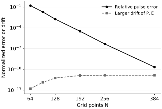
Small invariant drift does not imply an accurate KdV profile. These quantitative curves use the table above, with $\kappa=1$, $x_0=-2$, $T=1$, $\ell=48$ and $h=1/3200$. The dashed curve is the larger normalized drift of $P$ and $E$ over the sampled time steps. The vertical axis is logarithmic; the lines only connect tested resolutions.

Enlarge the domain at fixed spacing

Finally hold $\Delta x=1/8$ and $h=1/3200$ fixed, increasing $N$ with $\ell$.

Period length $\ell$	Grid points $N$	$\epsilon_2$	$\epsilon_\infty$
16	128	$1.37\times10^{-5}$	$2.33\times10^{-5}$
24	192	$4.73\times10^{-9}$	$7.81\times10^{-9}$
32	256	$2.08\times10^{-10}$	$2.35\times10^{-10}$
48	384	$2.17\times10^{-10}$	$2.40\times10^{-10}$

The initial/final endpoint values, as fractions of the pulse height, fall from $2.46\times10^{-5}$ at $\ell=16$ to $3.11\times10^{-19}$ at $\ell=48$. The last two errors form a floor set by remaining time and spatial errors. Their small difference does not establish that the smaller box is more accurate in general. Holding $N$ fixed while enlarging the box would coarsen $\Delta x$ and mix two effects.

The separate reference run at $\ell=48$, $N=512$ and $h=1/3200$ has $\epsilon_2=1.80\times10^{-10}$ and $\epsilon_\infty=1.87\times10^{-10}$. Its largest normalized integral drift is $1.39\times10^{-11}$.

A false solution with perfect line integrals

Translate the correct shape at half the correct speed:

$$u_{\mathrm{wrong}}(x,t)=2\kappa^2 \operatorname{sech}^2\!\left[\kappa(x-2\kappa^2t-x_0)\right].$$

Translation leaves $M,P,E$ unchanged, yet substitution gives

$$(u_t+6uu_x+u_{xxx})_{\mathrm{wrong}} =2\kappa^2(u_{\mathrm{wrong}})_x,$$

which is nonzero. At $T=1$, its relative $L^2$ error is $1.23$, while the three sampled integrals differ from the exact line values by at most $1.4\times10^{-16}$ relative. This deliberately incorrect trajectory shows why an equation residual or independent solution comparison is indispensable.

Exercises

Guided: measure the order

Using the last two temporal $L^2$ errors, compute the observed order and predict the error after one more halving if fourth-order behavior dominates. State one reason the prediction can fail.

Hint

Divide the errors, take the base-two logarithm, then use a factor of $2^4$ for the prediction.

Solution

The ratio is about $17.9$, giving order $4.16$. Fourth-order scaling predicts $7.42\times10^{-9}/16\approx4.64\times10^{-10}$. A remaining spatial, domain or roundoff error can spoil this scaling; the coefficient can also change before the asymptotic regime is reached. An observed order is evidence about this refinement, not an exact law for every step size.

Independent: expose the conservation blind spot

Use the $N=64$ spatial result to assess the claim: “The pulse is accurate to twelve digits because its conserved quantities drift by less than $10^{-12}$.” Distinguish the initial projection, the finite Fourier evolution and the continuum solution.

Hint

Inspect the profile error and the separate initial-projection fields in the saved JSON. Conservation measures change along a trajectory, not its distance from the requested trajectory.

Solution

The claim is false: the final profile has relative $L^2$ error about $0.162$. Projection discards high Fourier modes before time stepping. The retained system then evolves different finite-dimensional data and can nearly preserve its own discrete integrals. Neither that preservation nor agreement of a few initial integrals bounds the full field error. The spatial-refinement comparison directly tests the lost-resolution effect.

Transfer: resolve a narrower pulse

Change $\kappa$ from $1$ to $2$. How should spatial resolution, time interval and time step scale to compare the same dimensionless motion? Explain why doubling $N$ alone is insufficient.

Hint

Use $X=\kappa x$, $\tau=\kappa^3t$ and $u=\kappa^2U$.

Solution

To keep the scaled grid and motion fixed, halve $\Delta x$, divide $T$ and $h$ by eight, and halve the period length and initial center when scaling the whole physical setup. Equivalently, on an unchanged large box one needs at least twice as many points to keep the same points per width, while still refining time for the eightfold nonlinear/dispersive time scale. Doubling $N$ alone leaves the temporal and domain comparisons uncontrolled. Run new separate refinements; the saved acceptance results cover the original parameter set.

References

• Kassam, Aly-Khan, and Lloyd N. Trefethen. “Fourth-order time-stepping for stiff PDEs.” SIAM Journal on Scientific Computing 26(4), 1214–1233 (2005). DOI. Open PDF.