What makes a system integrable?

An integrability claim should tell you which mathematical structure makes a problem tractable. For a finite Hamiltonian system, there is a precise criterion involving enough independent, mutually commuting conserved quantities. Wave equations and quantum chains require their own stated structures. This first encounter begins with a nonlinear oscillator: its conserved energy determines the allowed motion even though the equation is not linear. You will calculate turning points, recognize an insufficient integrability argument, and choose an example to investigate further.

Required background. Squares, fourth powers and coordinates on a graph. Rates of change are introduced below; the calculus checks are explained where they occur.

Helpful background. Differential equations & phase portraits explains how an equation and initial data specify motion. It is available as a repair, not a prerequisite for the energy calculations here.

A nonlinear oscillator with a conserved energy

Consider a particle with dimensionless position $q(t)$, momentum $p(t)$ and time $t$, with mass and the force coefficient normalized to one. Its state is the pair $(q,p)\in\mathbb R^2$. Let

$$\dot q=p,\qquad \dot p=-q^3.$$

A dot means rate of change with time: the first equation identifies $p$ with velocity; the second gives a restoring force toward $q=0$. Unlike a harmonic oscillator, whose restoring force is proportional to $q$, this force is proportional to $q^3$.

The energy is

$$H(q,p)=\frac{p^2}{2}+\frac{q^4}{4}.$$

The first term is kinetic energy and the second is potential energy. As the particle moves, these terms change, but their sum stays fixed. A function of the state with this property is a conserved quantity, also called a first integral.

Calculus check: why this energy is conserved

The chain rule says to differentiate each changing term and multiply by the rate of its argument:

$$\frac{dH}{dt} =p\dot p+q^3\dot q =p(-q^3)+q^3p=0.$$

This is an identity at every state, not a check at one sampled time. The motion is Hamiltonian: $\dot q=\partial H/\partial p$ and $\dot p=-\partial H/\partial q$. A partial derivative varies the indicated coordinate while holding the other one fixed. The Hamiltonian bridge develops these rules.

Entry check: an energy is not a complete initial state

Calculate $H$ at $(q,p)=(1,0)$ and at $(q,p)=(0,1/\sqrt2)$. Are they the same state? Does specifying the energy alone tell you the particle’s initial position and direction of motion?

Repair: distinguish a value from the states having that value

Both have energy $1/4$:

$$H(1,0)=\frac14, \qquad H(0,1/\sqrt2)=\frac12\left(\frac1{\sqrt2}\right)^2=\frac14.$$

They are different states. The first is at rest at a positive turning point; its negative acceleration starts motion back toward the center. The second is already moving right through $q=0$. Energy selects a curve of possible states, not a single point. An initial state selects where on that curve the motion begins.

Read the motion from an energy curve

Take $H=E=1/4$. Rearranging the energy equation gives

$$p^2=\frac{1-q^4}{2}, \qquad p=\pm\sqrt{\frac{1-q^4}{2}}.$$

Real momentum requires $-1\le q\le1$. These two branches join at $(q,p)=(\pm1,0)$, forming a closed curve in the position–momentum plane.

Position	Possible momentum	Meaning for the motion
$q=-1$	$p=0$	Left turning point; $\dot p=1$ sends the particle right.
$q=0$	$p=\pm1/\sqrt2$	Crossing the center, in either direction.
$q=1$	$p=0$	Right turning point; $\dot p=-1$ sends the particle left.

On the upper branch $p\gt0$, so $\dot q\gt0$: the particle moves right. On the lower branch it moves left. The smooth vector field never vanishes on this curve, and the motion repeats around it. The equilibrium $(0,0)$ lies on the different energy level $E=0$.

The exact curve below shows both branches and the direction of motion. Its points represent position and momentum together; it is not a plot of position against time.

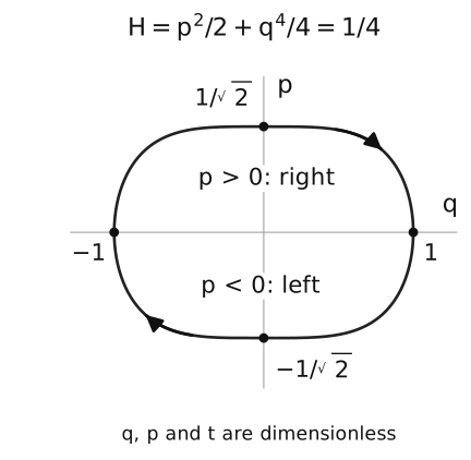
Exact $H=1/4$ level for $H=p^2/2+q^4/4$, with dimensionless $q,p,t$. Dots mark turning points $(\pm1,0)$ and center crossings $(0,\pm1/\sqrt2)$; arrows follow $\dot q=p$ and $\dot p=-q^3$. The origin belongs to the separate level $H=0$.

For general $E\gt0$, exactly the same algebra gives the turning-point magnitude and maximum momentum:

$$a=(4E)^{1/4},\qquad |q|\le a,\qquad |p|\le\sqrt{2E}.$$

The maximum momentum occurs at $q=0$, where all the energy is kinetic. At $q=\pm a$ it is all potential. These are exact consequences of the conserved quantity.

Optional calculus: recovering time by one integral

On a right-moving segment, $p=\dot q=\sqrt{2E-q^4/2}$. Therefore

$$t-t_0=\int_{q_0}^{q(t)}\frac{ds}{\sqrt{2E-s^4/2}}, \qquad -a\lt q_0\le q(t)\lt a.$$

This is a quadrature: time is obtained from a specified integral. For $E=1/4$, it becomes $\sqrt2\int_{q_0}^{q(t)}ds/\sqrt{1-s^4}$. We have not needed an elementary sine or exponential formula for $q(t)$.

This branch formula does not describe a complete oscillation by itself. At the right turning point, continue on the branch with negative momentum. The time to reach that point is finite: the denominator vanishes like a constant times $\sqrt{a-s}$, whose reciprocal has a finite integral up to $a$. Symmetry gives the full period

$$T(E)=4\int_0^a\frac{ds}{\sqrt{2E-s^4/2}} =4E^{-1/4}\int_0^1\frac{dr}{\sqrt{1-r^4}}.$$

The last equality follows by $s=ar$, with $a=(4E)^{1/4}$. Unlike the harmonic oscillator, this oscillator has an energy-dependent period. The smooth equations, together with bounded motion on the energy curve, supply the continuation through each turning point.

When are conserved quantities enough?

One position–momentum pair is one degree of freedom, although its state needs two numbers. For $n$ degrees of freedom, use $n$ positions and $n$ momenta, so phase space has dimension $2n$.

For a smooth, time-independent Hamiltonian system in these canonical coordinates, Liouville integrability requires $n$ conserved functions, including $H$, with two properties:

• They are independent on an open dense regular set: their differential gradients have rank $n$, rather than repeating the same constraint.
• They are in involution: every pair has zero Poisson bracket, the Hamiltonian compatibility condition defined below.

This is the classical definition in Cannas da Silva, January 2006 revision, § 18.4, pp. 109–110, Definition 18.10, PDF. The integrability reference states its geometric scope more fully.

Optional calculus: the compatibility test

For functions $F$ and $G$ of the canonical coordinates, define

$$\{F,G\}=\sum_{i=1}^n \left( \frac{\partial F}{\partial q_i}\frac{\partial G}{\partial p_i} -\frac{\partial F}{\partial p_i}\frac{\partial G}{\partial q_i} \right).$$

For a function with no explicit time dependence, its rate along Hamiltonian motion is $dF/dt=\{F,H\}$. Conservation therefore requires $\{F,H\}=0$. Involution additionally requires $\{F_i,F_j\}=0$ for every pair among the chosen functions. Several quantities can each be conserved without satisfying this pairwise condition. See the worked examples in the bracket bridge.

Our quartic oscillator has $n=1$, so $H$ alone supplies the required count. Its gradient is $(q^3,p)$, nonzero everywhere except the equilibrium. A function always has zero bracket with itself, so $\{H,H\}=0$. The system is Liouville integrable, with regular positive-energy curves and a singular zero-energy equilibrium.

It is nevertheless nonlinear. Doubling a nonzero solution’s position doubles its acceleration, while the cubic force would become eight times as large. Thus a doubled motion is generally not another solution. Nonlinearity does not obstruct the conserved-energy calculation or the integrability criterion.

For more degrees of freedom, one conserved energy is generally insufficient to establish the required structure. Also, the criterion alone does not make every orbit periodic. Compact, connected, regular common levels give the torus setting of the Liouville–Arnold theorem; motion on a higher-dimensional torus can be quasiperiodic. Compactness and regularity are additional hypotheses for that conclusion.

What changes for waves, quantum states and probabilities?

The classical criterion counts functions on a finite-dimensional phase space. Applying the same words elsewhere requires stating which structure is meant.

For KdV waves, one exact travelling pulse is a solution for particular data. The two-soliton collision establishes more: an interacting field recovers two outgoing pulses with the original amplitudes and speeds but shifted positions. Inverse scattering explains this family by evolving and reconstructing spectral data. A general inverse-scattering theorem needs analytic hypotheses beyond that explicit calculation; see Aktosun 2009, §§ III and IX. One attractive wave plot alone establishes none of those broader claims.

For the quantum XXX chain, the site constructs transfer matrices, a family of operators depending on a parameter. Their pairwise commutation and relation to the Hamiltonian are proved from a local algebraic identity. That construction supplies useful structure across chain sizes. Merely saying that some conserved operators commute would be too weak: every finite Hermitian matrix has commuting projectors onto an eigenbasis. Numerical diagonalization therefore cannot, by itself, distinguish this integrable structure. Caux and Mossel, § 3, pp. 4–7 of arXiv v1, PDF explain this problem with a naive quantum definition. The reference gives the projector calculation explicitly.

For stochastic particle motion, an exact stationary distribution answers a steady-state question. It does not automatically determine the full time-dependent distribution from every initial state. The finite-ring TASEP entrance separates the stationary current, a particular Bethe decay mode, and numerical checks against finite-state evolution. Each calculation has a stated scope.

Thus linearity concerns the form of an equation and superposition; an exact solution concerns a specified problem; and integrability concerns a stated mathematical structure. None of those labels can replace the other two.

Exercises

Guided: change the oscillator’s energy

For $H=p^2/2+q^4/4$, set $E=4$. Find the two turning positions and the largest possible $|p|$. Compare them with the $E=1/4$ example. Is a negative energy allowed? Why does the pair $(q,p)$ still describe only one degree of freedom?

Hint

At a turning point $p=0$. At maximum momentum $q=0$. Both terms of $H$ are nonnegative.

Solution

The turning points obey $q^4/4=4$, so $q=\pm2$. The largest momentum obeys $p^2/2=4$, so $|p|=2\sqrt2$. Increasing the energy from $1/4$ to $4$ doubles the turning-point magnitude and quadruples the maximum momentum. Negative energy is impossible for real $q,p$. There is one position coordinate and its conjugate momentum; degrees of freedom count these pairs, not individual phase-space coordinates.

Independent: do two formulas give two integrals?

A two-degree-of-freedom Hamiltonian system has conserved energy $H$. A calculation lists $F_1=H$ and $F_2=H^2$ and declares Liouville integrability because there are two conserved formulas. Assess the argument. What information is still needed, and does the failed argument prove that the system is nonintegrable?

Hint

If $H=E$ is known, can the value of $H^2$ still vary independently? For a calculus check, differentiate $H^2$.

Solution

The second formula adds no independent constraint: $H=E$ already implies $H^2=E^2$. Precisely, $d(H^2)=2H\,dH$, so the two gradients never have rank two. The functions commute, but independence fails. To establish the stated criterion, find another conserved function independent of $H$ on an appropriate open dense regular set and check its bracket with $H$. This unsuccessful choice does not prove that no such function exists. It leaves integrability undecided.

Transfer: add damping and recheck the claim

Change the oscillator to

$$\dot q=p,\qquad \dot p=-q^3-\gamma p, \qquad \gamma\gt0.$$

Use the energy calculation above to find $dH/dt$. At $(1,0)$ this derivative vanishes instantaneously: does that make $H$ conserved? Explain which earlier argument fails and why this does not settle every possible meaning of integrability for the modified equation.

Hint

Insert the new $\dot p$ into $p\dot p+q^3\dot q$. At $(1,0)$, also calculate $\dot p$ to see whether the momentum remains zero.

Solution

The rate is

$$\frac{dH}{dt} =p(-q^3-\gamma p)+q^3p=-\gamma p^2.$$

Energy decreases whenever $p\ne0$. At $(1,0)$, $\dot p=-1$, so the particle immediately develops nonzero momentum; a zero instantaneous energy derivative is not a conserved-energy identity. The old positive-energy curves are no longer invariant, and the displayed $H$ no longer generates the modified motion through the same canonical Hamilton equations. Our proof of Liouville integrability therefore does not apply. Failure of that proof is not a theorem excluding every alternative structure or solution method for this different system.

Choose the calculation you want to understand

To continue with the quartic oscillator used here, Build actions and angles derives its exact action and period. It then constructs a uniformly advancing angle around the nonlinear energy curve, explaining why the frequency depends on energy.

• Particles and conserved quantities: start with open Toda, where the work is to establish enough independent commuting integrals for a chain, beyond the one-degree-of-freedom example here.
• Quantum states and scattering: start with the XXX chain, then connect explicit spin states to the commuting-transfer construction.
• Nonlinear waves and collisions: start with KdV, deriving a pulse before its spectral reconstruction and two-soliton interaction.
• Random motion and exact probabilities: start with the Markov bridge, then calculate the stationary current and a finite-ring relaxation mode for TASEP.

Choose one object and a calculation whose result you can check. As the methods become more powerful, keep asking which data, boundaries and observables the result actually covers.

References

• Aktosun, Tuncay. “Inverse Scattering Transform and the Theory of Solitons.” In Robert A. Meyers (ed.), Encyclopedia of Complexity and Systems Science. Springer, 2009, pp. 4960–4971. DOI. Author version arXiv:0905.4746v1; open text, §§ III and IX.
• Cannas da Silva, Ana. Lectures on Symplectic Geometry. Lecture Notes in Mathematics 1764. Springer, 2001. DOI. Author revision January 2006, PDF, § 18.4, pp. 109–111.
• Caux, Jean-Sébastien, and Jorn Mossel. “Remarks on the notion of quantum integrability.” Journal of Statistical Mechanics: Theory and Experiment (2011), P02023. DOI. Author version arXiv:1012.3587v1, submitted 16 December 2010; PDF, § 3, printed pp. 4–7. This citation uses that version identity, not the later compilation date displayed by the PDF.